14 MTM HRMS Library: LC-HRMS

REWRITE SECTION TO ONLY USE DDA OR RUN BOTH DDA AND DIA?

THIS SECTION IS INCOMPLETE AND SOME TEXT AND FIGURES ARE COPIED FROM GC TUTORIAL. NEED UPDATE!

UNIFI SCIENTIFIC LIBRARY: https://support.waters.com/KB_Inf/UNIFI/WKB190999_How_to_build_and_manage_a_scientific_library_in_UNIFI

Please see the introductory section in the previous chapter regarding the MTM HRMS library using GC-HRMS.

For LC analysis, the chemical standards should be run using data dependent analysis (DDA) instead of data independent analysis (DIA). For our waters G2 XS qToF instrument, the MSe is equivalent to DIA. Main distinction of MSe is the use of a ramp of collision energy in the collision cell whereas other DIA methods use a fixed collision energy. Therefore the MS2 spectra between different instruments and collision energies will also differ, which makes spectral matching more challenging in LC-HRMS compared to GC-HRMS. It is therefore common to analys the same chemical standard using different collision energies to cover the different fragment spectra (MS2) for the same compound.

ADD MORE INFO ABOUT ADDUCT SELECTION

This tutorial will guide you through the different steps to export the spectra information for each compound from a standard to contribute to the MTM HRMS spectral library. The project is organized in different subfolders within the main folder folder named “MTM_HRMS_LIB”. Do not change the name of any folders.

We first start with the raw data file from the HRMS analysis of a standard and we want to generate a .msp file as a final file format. The msp file is a file format developed by NIST to store mass spectral data. For more information about this format, please see this document.

The overall goal can be seen in Figure @ref(fig:combineMSP)

At least one solvent blank needs to be analyzed together with the standards in order to subtract any blank signals at a later stage.

The main steps of this procedure can be seen in below Figure @ref(fig:LCdiagramSpeclib).

General workflow for spectral library

The template folder for the spectral library is organized as follows:

MTM_HRMS_LIB
│   MTMxxxxx_GC-EI-FT_POSITIVE.xlsx
|   MTMxxxxx_LC-ESI-QTOF_POSITIVE.xlsx
│   ..
└───0_Main_Lib
│   │   MTM_HRMS_MAINLIB.xlsx
│   │   ..
│   
└───1_Standard_infosheets
│   │   MTM00001_GC-EI-FT_POSITIVE.xlsx
│   │   MTM00002_GC-EI-FT_POSITIVE.xlsx
|   |   ..
│
└───2_mzML_data
│   └───GC_CI_NEG_HRMS
│   └───GC_CI_POS_HRMS
│   └───GC_EI_HRMS
|   └───LC_ESI_NEG_HRMS
│   └───LC_ESI_POS_HRMS
|
└───3_MSP
│   │   MTM00001_GC-EI-FT_POSITIVE_IASLDLGGHXYCEO-HWKANZROSA-N.msp
│   │   MTM00002_GC-EI-FT_POSITIVE_UPMLOUAZCHDJJD-UHFFFAOYSA-N.msp
│   │   ..
│
└───4_Massbank
│   │   MTM00001.txt
|   |   MTM00002.txt
|   |   ..
│
└───MSDIAL_PROJECT
|   └───MSDIAL_params
|   
└───R
    |   MTM_HRMS_database.Rmd

The main folder (MTM_HRMS_LIB) contain some template information sheet that are used to fill in information about the standard and the analysis method. The MTM id number (MTMxxxxx) for each standard infosheet is in numeric order and must contain 8 character in total. Check the MTM_HRMS_MAINLIB.xlsx for the latest id number and use the next one as the new MTM id.

INSTALL REQUIRED SOFTWARE

Several software and packages are needed to generate the spectra library. All are open access and free to use for academic purposes.

Proteowizard: We mainly use MSConvert which is bundled in the Proteowizard software package and you can download it here.
MS-DIAL: used to analyze the mzML file and generate spectra. Download the latest version here. No installation is necessary so you only need to extract the downloaded zip file to your folder of choice.
MS-FINDER: used to annotate the individual peaks in the spectrum and export to msp file.

14.1 Analyze the standards using HRMS

It is recommended to analyze single standards but mixtures are also feasible to analyze if the analytes are not coeluting too close to each other. The deconvolution algorithm of MS-DIAL is able to distinguish between two peaks that are closely eluted but still have slightly different retention times and peak shapes.
You should also inject a solvent blank to perform blank subtraction later in MS-DIAL.

14.2 Convert the raw data file from LC-HRMS in unifi to mzML using MSconvert

Please check the steps according to @ref(MSConvertunifi)

14.3 Fill in the standard infosheet

In the main folder, choose one of the standard information sheets depending on whether you used LC or GC and the ionization mode. The content of the information sheet looks slightly different depending on LC or GC. Copy the chosen infosheet to the “1_Standard_infosheets” folder. In that folder, rename the copied infosheet to the new MTM id as mentioned in previous section.
The infosheet is organized in accordance to the format used by Massbank Europe. A description on the Massbank record format can be found here. It is important that you do not change any of the titles in the first column in the infosheet, as the format requirement is quite strict. Also, try not to copy text from one cell to another as it might change the underlying format of the cells (if you think you made an error, copy the template and redo again).
The rows that are in bold are information that are mandatory to fill in.

The “ACCESSION” row is the MTM id.

The “RECORD_TITLE” will be automatically generated based on the information you filled in so you should not fill this row.

“COMMENT: centroided mzML file name” is for internal purposes and refers to the name of the mzML file you converted and copied to the “MTM_HRMS_LIB/2_mzML_data/../” folder.

“COMMENT: msp file name” is automatically generated and will be used later to name the msp file.

“COMMENT: CONFIDENCE” refers to how confident you are of the identification of your standard according to the “Schymanski scale”. Leave it as “Reference Standard (Level 1)”, unless there are standards where you cannot distinguish or identify between different isomers in a standard. In this case, you should use “Level 3”. An example is “Technical mixture (Level 3)”, where we analyzed a technical standard (usually <90% purity) and several isomeric peaks can be seen in the chromatogram. In this case, I usually individually register each isomer in its own infosheet.

“CH$NAME:” occurs twice which means you have to input two different names for the compound in the standard, because a compound can have different names. It could be the common name specified in PubChem, the IUPAC name, trade name or the abbreviation.

“CH$IUPAC” is the InChI and always starts with “InChI=”. You can find all these information for the compound by searching in PubChem.

For GC compounds, you also need to fill in the “AC$CHROMATOGRAPHY: KOVATS_RTI” and “AC$CHROMATOGRAPHY: RETENTION_TIME”. These will be available later in MS-DIAL.

The other rows should be quite straightforward to fill in. If you use the same method for many standards, then you can save a copy of an infosheet to use as a method template, while only updating information for each specific compound: ACCESSION, DATE, COMMENT: centroided mzML file name, CH$NAME, CH$NAME, CH$FORMULA, CH$EXACT_MASS:, CH$SMILES:, CH$IUPAC:, CH$LINK: CAS, CH$LINK: INCHIKEY

The AC$CHROMATOGRAPHY: RETENTION_TIME row will be obtained later using MS-DIAL.

Now that you have filled in most information about the compound, we can proceed to process the mzML file to extract the spectra using MS-DIAL (although you can also first process the mzML files and then fill in the information afterwards).

14.4 Use MS-DIAL to perform spectral deconvolution and generate spectra for each compound

The graphical user interface of MS-DIAL takes some time to get used to since it is centered around detected peaks. It is important that you choose the correct parameters in the beginning since the parameters can affect the peak detection and alignment, or else you need to redo the data preprocessing again which could take long time if you are analyzing a lot of samples. When you run a large number of real samples, it is recommended to first optimize the parameters using e.g. QC samples. In this case where we analyze standards, then the default parameters with some instrument specific parameters can be used. These are found in the subfolder MSDIAL_PROJECT/MSDIAL_params/. If you want to know more details about data processing using MS-DIAL, please check the MS-DIAL online tutorial.

The below steps are based on the workflow for GC-EI orbitrap data described by Price et al. and adapted to LC-HRMS.

IN THIS EXAMPLE HERE, I WILL USE ONE STANDARD OF PFAS ANALYZED IN LC-ESI IN POSITIVE MODE

1. In the File menu, start a new project. You must choose a file path where the mzML file(s) are located. When the data analysis is finished, several files associated with the analysis is created in the same folder. Depending on GC or LC analysis, then different parameters needs to be selected. Below Figure @ref(fig:LCMSDIALStartup) shows parameters for LC analysis. LC-ESI is a soft ionization and the Waters G2 XS qtof instrument uses MSe which has an alternating low energy scan and high energy scan. Choose “SWATH-MS” and then browse to the _“MSDIAL_PROJECT_params*MSe_50_1200_params.txt”* file. This specifies the parameters for the MSe experiment. Since we also centroided the mzML file for both MS1 and MSMS so these parameters needs to be specified. In this example, we ran a PFAS standard in negative mode, so this ion mode was choosen in this case.

Click on the “Advanced: add further meta data” tab. The information for different instruments in our lab can be found in the file “/MTM_HRMS_LIB/MSDIAL_PROJECT/MSDIAL_params/Metadata.txt”. If your instrument is not present then you can input these by yourself. This metadata is optional but the information will be added to the msp file later.
When you are finished, click on next.

2. Click on the browse button and then you will select the files to process. The default file format is .abf but we want to process .mzML so choose this file format instead. You will now see the mzML file(s) in your working directory. If you want to process multiple files use Shift/Ctrl + select. Make sure your standards are designated as “Sample”. You should include a solvent blank which will be designated as “Blank”. The other columns are for post processing and not important for this spectral database workflow. You can learn more about these in the tutorial.

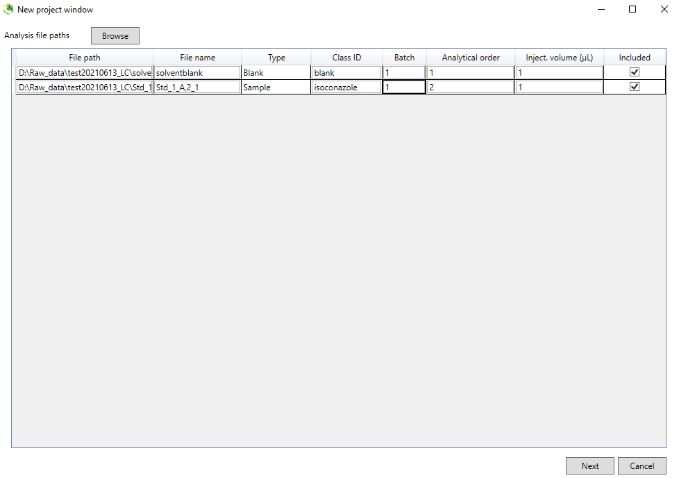
Click on next to the Analysis parameter settings.

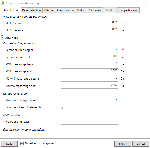
3. The following instructions are for Waters G2 XS qtof in ESI negative mode, but the other processing methods are similar. Below Figure @ref(fig:LCMSDIALPeakdetection) shows the parameters for the XS qtof instrument. The MS1 and MS2 tolerance was set to 0.05 Da. Click on the “Advanced” tab and check the “Consider Cl and Br elements”. You can also choose how many samples (threads) to process in parallel.

Continue with the “Peak detection” tab and set an appropriate minimum peak height. Use the following parameters for our spectral library purpose:
Minimum peak height: 1000 amplitude.
Mass slice width: 0.05 Da.

This is instrument specific and also depends on the concentration of the analytes. The advanced tab can be left as default.

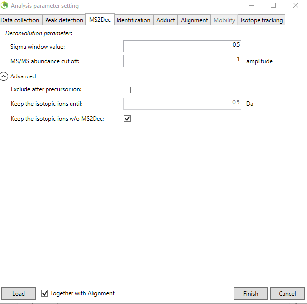
Continue to the “MS2Dec” tab.

4. The sigma window value is an important parameter which determines the efficiency of the deconvolution algorithm. The parameter depends on the instrument and Figure @ref(fig:LCMSDIALMS2Dec) shows the recommended ones for the GC orbitrap analysis of standards. From the online tutorial: “The sigma window value is highly affected by the resolution of deconvolution. A higher value (0.7-1.0) will reduce the peak top resolutions, i.e. the number of resolved chromatographic peaks will be decreased. On the other hand, a lower value (0.1-0.3) may also recognize many noise chromatographic peaks..”

The “Identification” tab is not necessary to modify for our purpose and mainly important when processing real samples (using the HRMS library as suspect list).

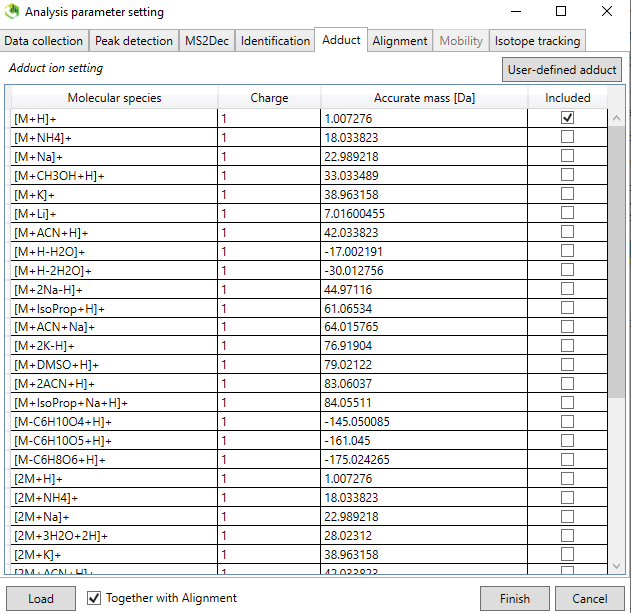
Go on to the “Adduct” tab.

__5._ The adduct should be chosen based on your knowledge of the ionization behavior of the standards. Most common is the [M-H]- ion for negative mode and [M+H]+ ion for positive mode. some compounds have much higher ion abundance for other adducts and therefore these can be included also. You also define your own adducts in the “User-defined adduct” subtab if it is not present in the list.

“Alignment” tab. The purpose of alignment is to align all individual samples so the retention times for the same for the same compound between all samples. This is because the chromatographic separation will change between runs and batches and needs to be aligned. In the “Advanced” subtab, check the “Remove features based on blank information”. A sample/blank ratio of 5 should be ok. This will remove any features that are lower than five times the blank samples (solvent blank in this case). Everything else can be as default.

The “Isotope tracking” tab does not need to be modified in this workflow.

Press Finish and the process will begin. This might take some time depending on how many samples you are processing and the processing power of the computer.

Now you are done and click on “Finish”.

After the peak detection and deconvolution process is finished, you should see below screen.

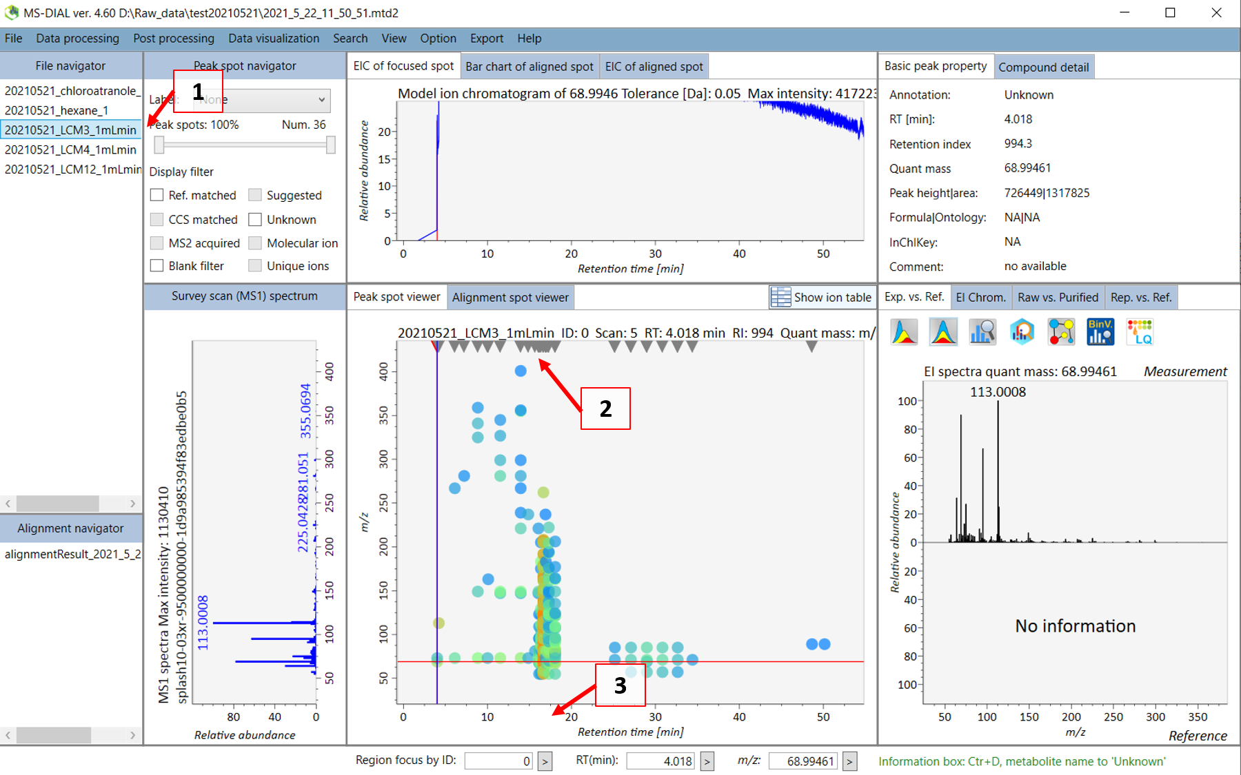
Double click on the sample name where your standard was analyzed (see 1 in Figure @ref(fig:LCMSDIALSample)). Your screen will be switched to the “Peak spot viewer” tab. Each detected component will be seen as a downward pointing triangle (see 2 in Figure @ref(fig:LCMSDIALSample)). You should zoom in to the peak by moving you pointer to below the x-axis and scroll to zoom in the retention time axis (3). You should now be able to see the peak more clear and click on the peak as seen in 4 in Figure @ref(fig:LCMSDIALPeak).

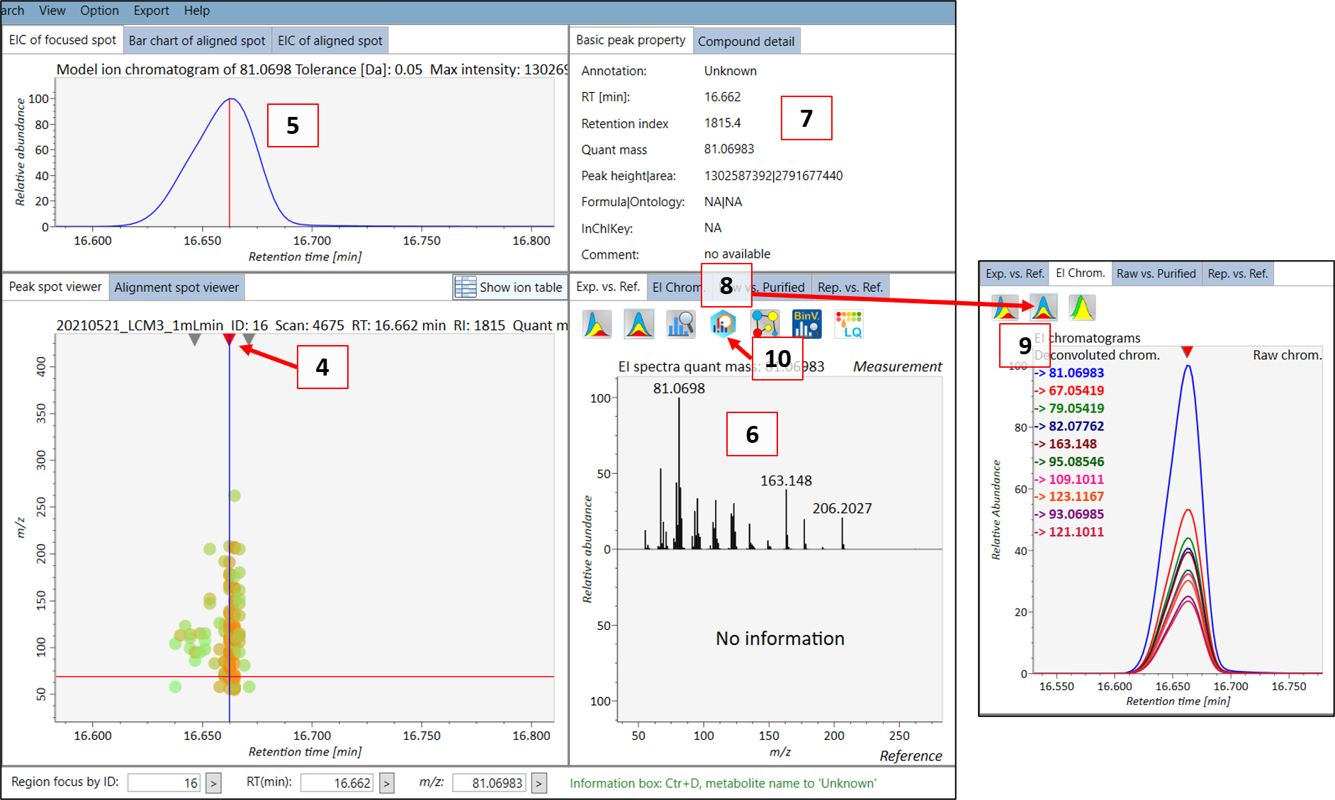
You can then see the EIC (5) of the chosen peak to check if the peak shape is good. The extracted spectrum will be shown in (6), and the retention time and retention index can be seen in (7). This is the deconvoluted spectrum and you can see the peak shape of the ion fragments with the highest intensities by choosing the “EI chrom” tab (8) which allows you to see if the deconvolution process has been successful (9). When you feel that the quality is good, then you can export the spectrum to MS-FINDER by clicking on the “MS FINDER search” button (10).

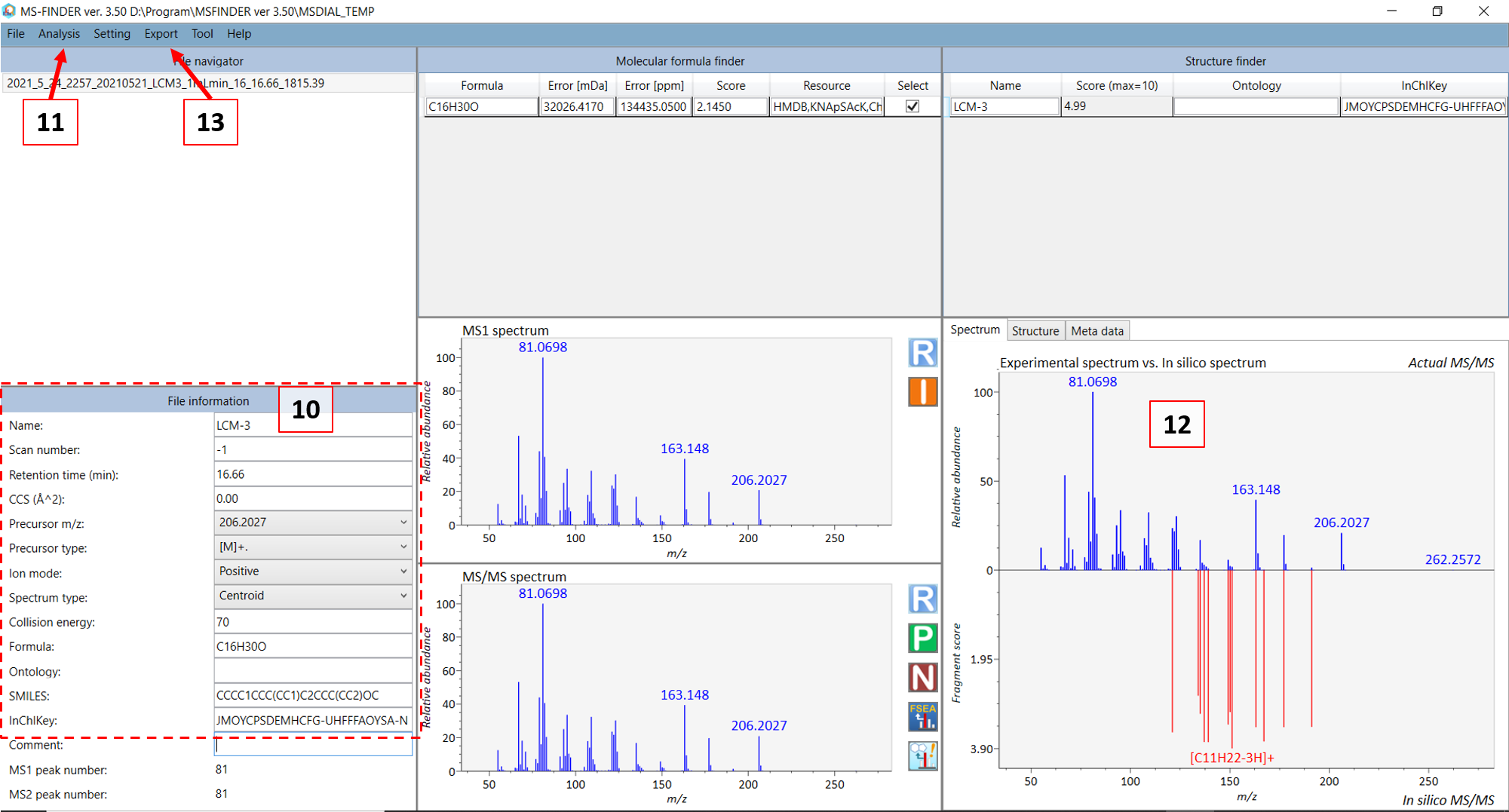
In the new MS-FINDER window, fill in the information in (10) in Figure @ref(fig:LCMSFINDER) for your compound. For GC-MS, in most cases the monoisotopic peak (somewhat equivalent to the precursor ion in LC mode) and you can choose the ion closest to the monoisotopic mass of your standard compound. Then choose the precursor type. For GC-MS: choose [M]+. (M plus dot). After you are done, select “Fragment annotation (single)” in the ““Analysis” menu (11). Afterwards, select the “Fragment annotation (batch job)” under the same menu. The in silico annotation of the fragment ions should now be calculated (12) and you can thereafter export the annotated spectrum as an “.msp” file (see 13). Use the file name that was generated in the standard infosheet you filled at the “COMMENT: msp file name” row. Save the file in the “3_MSP” subfolder.

Now you are finished with generating the msp file for your standard spectrum.

Send the newly created files together with the mzML files to Thanh

The mainlib excel file as well as the combined msp file will be updated on a regular basis or upon request.

The final msp file will look something like below (not including the ## sign). A note is that the retention index is not included by MS-FINDER when you export to msp file. This will be later automatically added to the combined database based on the retention index value in the infosheet for the specific standard. Therefore, it is important to check that all files have consistent MTM IDs for the same measured compound.

NEED TO UPDATE TO LC msp